
Blank Seismic Tripartite Graph Paper
I had a project for work a couple years ago where I needed to plot a seismic response on tripartite paper, but any of the blank tripartite paper I could find (online or in books) was of low quality. I enlisted the help of tex.stackexchange and engineering.stackexchange to see if anyone had a method for generating such paper, and got a couple good answers.
Recently I had another similar project and happened to figure out a solution using LaTeX that I thought was worth sharing. LaTeX is my preferred method for authoring academic-type papers, since it can create some truly beautiful results. Take for example the response spectra plot below of the 1952 Taft Earthquake (data retrieved from the PEER Strong Ground Motion Database), which I plotted over one of my tripartite graphs. Absolutely gorgeous.

The method for creating such tripartite paper doesn’t seem to be widely published (at least, not online), so I’ll go through the process now. If you don’t care about the process, scroll to the bottom for a PDF file with seismic tripartite graphs in the frequency and period domain, in both US customary and metric units.
The axes for acceleration and displacement are not an arbitrary size. Referring to Eqns. 5.20 and 5.21 of Structural Dynamics: Theory and Computation, 5th Ed. by Paz and Leigh, the lines for constant acceleration or displacement can be plotted as
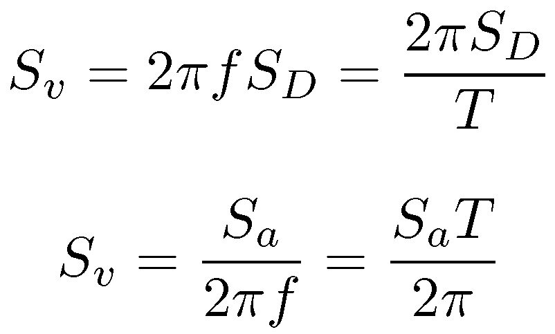
The range for these will vary depending on the limits of the x and y axes. Plotting these lines is pretty trivial, if repetitive, but they are missing any kind of helpful labeling for the acceleration and displacement values.
We now need to plot nodes with labels in PGF/TikZ. Essentially what we’re doing is making a scatter plot with invisible data points, which serve as the anchor for the label. The label has a rotation to match the skew of the secondary axes. Trying to figure out these node coordinates in terms of frequency/period and pseudo velocity by trial an error is a pain, but it’s relatively easy to figure out where they need to go based on the acceleration and displacement. Knowing these, the frequency or period associated with that point can be found by combining the above equations and solving for f or T, as
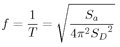
Then, the pseudo velocity associated with this frequency and acceleration/displacement can be found using one of the previous equations. This sort of process lends itself to a spreadsheet, which I have created and have linked below for use. With the line labels created, the tripartite graph is done.

If you’re interested in generating these tripartite graphs for yourself using LaTeX, the files for this are included below for download. These are released under the Creative Commons Attribution-NonCommercial-ShareAlike 4.0 International (CC BY-NC-SA 4.0) license.
Files
PDF file of tripartite graphs (frequency and period domains, US customary and metric units)
TeX file that generates the above PDF
Excel file for location acceleration and displacement line label anchors in PGF/TikZ
If you have any questions, comments, or suggestions for improvement, please email me. If you have questions on using LaTeX, you’re better off asking your questions on Stack Exchange since I’m not much of a power user. Any requests to create a custom graph for you will be ignored unless there’s a reasonable monetary offer made 😀